Investigating Block Cipher Modes with DPA
Block Cipher Modes
In the real world, it's a bad idea to encrypt data directly using block ciphers like AES. The goal of encryption is to produce ciphertexts that look pseudo-random: there should be no visible patterns in the output. Using a block cipher directly, encrypting the same plaintext multiple times will always result in the same ciphertext, so any patterns in the input will also appear in the output. This encryption method is called the Electronic Code Book (ECB) block cipher mode.
To get around the weaknesses of ECB mode, there are alternative encryption methods that reuse the basic block ciphers and their core. A number of these are described on Wikipedia. On top of ECB mode, there are 4 more block cipher modes that this attack will consider.
Cipher Block Chaining (CBC): The plaintext is XORed with the previous ciphertext before being encrypted. There is no ciphertext before the first plaintext, so a randomly chosen initialization vector (IV) is used instead:
Cipher Feedback (CFB): The previous ciphertext is used as the input for the cipher. Then, the plaintext is XORed with the result to get the new ciphertext. Again, an IV is used to replace the missing ciphertext:
Output Feedback (OFB): An IV is repeatedly encrypted to produce a pseudo-random sequence of blocks. Then, these encryption results are XORed with the plaintexts to produce the ciphertexts:
Counter (CTR): An incrementing counter is encrypted to produce a sequence of blocks, which are XORed with the plaintexts to produce the ciphertexts:
All four of these modes share the same quality: if the same plaintext block is encrypted multiple times, the result will be different every time. The goal of this attack is to take a target that's using one of these five cipher modes and determine which mode is being used.
Firmware
To perform this attack, the SimpleSerial AES XMEGA firmware was modified to allow the target to use all five of these block cipher modes. The encrypt() function takes a new plaintext and produces the next ciphertext:
void encrypt(uint8_t* pt)
{
	static uint8_t input[16];
	static uint8_t output[16];

	// Find input
	switch(BLOCK_MODE)
	{
		case ECB:
			for(int i = 0; i < 16; i++)
				input[i] = pt[i];
			break;

		case CBC:
			for(int i = 0; i < 16; i++)
				input[i] = pt[i] ^ ct[i];
			break;

		case CFB:
			for(int i = 0; i < 16; i++)
				input[i] = ct[i];
			break;

		case OFB:
			for(int i = 0; i < 16; i++)
				input[i] = output[i];
			break;

		case CTR:
			input[0]++;
			break;
	}

	// Encrypt in place
	for(int i = 0; i < 16; i++)
		output[i] = input[i];
	aes_indep_enc(output);

	// Use output to calculate new ciphertext
	switch(BLOCK_MODE)
	{
		case ECB:
		case CBC:
			for(int i = 0; i < 16; i++)
				ct[i] = output[i];
			break;

		case CFB:
		case OFB:
		case CTR:
			for(int i = 0; i < 16; i++)
				ct[i] = output[i] ^ pt[i];
			break;
	}
}
Check that all five of these modes match the diagrams above. Note that there is no way to select an IV in this code - the contents of ct[] are not fixed when the target is powered on. However, the IV isn't important for these attacks, so this limitation isn't a big deal.
This code was compiled five times with five different values of BLOCK_MODE, producing five hex files (one for ECB encryption, one for CBC, etc). All of this code is in the ChipWhisperer repository under chipwhisperer\hardware\victims\firmware\simpleserial-aes-modes\.
Captures and Attack
To perform the attack, each of the five hex files were loaded onto the ChipWhisperer Lite XMEGA target. Then, 200 traces were captured for each block cipher mode, using a fixed key and random plaintexts. All of the NumPy data files were copied from the project folder so they could be loaded in a Python script.
To tell the difference between the five cipher modes, DPA was used to search for the input to the AES encryption function. Recall that all five of the modes combine the plaintexts and ciphertexts in different ways to calculate the input blocks. The input for each mode uses:
| Mode | Plaintext | Ciphertext |
| ECB | Current | — |
| CBC | Current | Previous |
| CFB | — | Previous |
| OFB | Previous | Previous |
| CTR | — | — |
Using this information, the DPA attack uses the following steps:
- Use the current/previous plaintexts and ciphertexts to calculate four different possible AES inputs (the inputs for ECB, CBC, CFB, and OFB modes)
- For each of these calculated inputs, use one bit of the input to split the traces into two groups
- Calculate an average trace for each group and subtract them to get four differential traces
- Look at the differences to decide which mode is most likely:
- If one of the differential traces shows a large spike, the target is probably using that mode
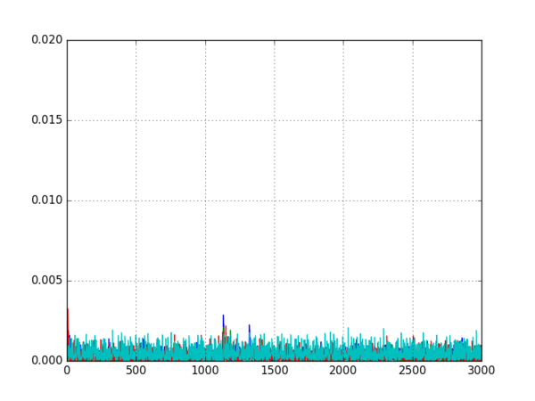
- If none of the differential traces has a large spike, the target is probably using CTR mode
A simple Python script to implement this attack is:
import numpy as np
import matplotlib.pyplot as plt

# Load data
pt     = np.load('traces/ecb_textin.npy')
ct     = np.load('traces/ecb_textout.npy')
traces = np.load('traces/ecb_traces.npy')
numtraces = np.shape(traces)[0]

# Create groups for all 4 modes
grouped_ecb = [[] for _ in range(2)]
grouped_cbc = [[] for _ in range(2)]
grouped_cfb = [[] for _ in range(2)]
grouped_ofb = [[] for _ in range(2)]

# Sort traces into groups
for i in range(1, numtraces):
    bit_ecb = (pt[i][0]               ) & 0x01
    bit_cbc = (pt[i][0]   ^ ct[i-1][0]) & 0x01
    bit_cfb = (ct[i-1][0]             ) & 0x01
    bit_ofb = (pt[i-1][0] ^ ct[i-1][0]) & 0x01

    grouped_ecb[bit_ecb].append(traces[i])
    grouped_cbc[bit_cbc].append(traces[i])
    grouped_cfb[bit_cfb].append(traces[i])
    grouped_ofb[bit_ofb].append(traces[i])

# Calculate means
means_ecb = [np.average(grouped_ecb[0], 0), np.average(grouped_ecb[1], 0)]
means_cbc = [np.average(grouped_cbc[0], 0), np.average(grouped_cbc[1], 0)]
means_cfb = [np.average(grouped_cfb[0], 0), np.average(grouped_cfb[1], 0)]
means_ofb = [np.average(grouped_ofb[0], 0), np.average(grouped_ofb[1], 0)]

# Plot differences
plt.plot(abs(means_ecb[1] - means_ecb[0]))  # Blue
plt.plot(abs(means_cbc[1] - means_cbc[0]))  # Green
plt.plot(abs(means_cfb[1] - means_cfb[0]))  # Red
plt.plot(abs(means_ofb[1] - means_ofb[0]))  # Teal
plt.axis((0, 3000, 0, 0.02))
plt.grid()
plt.show()
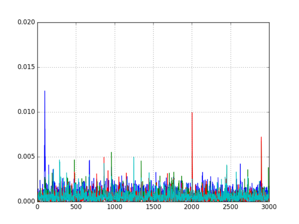
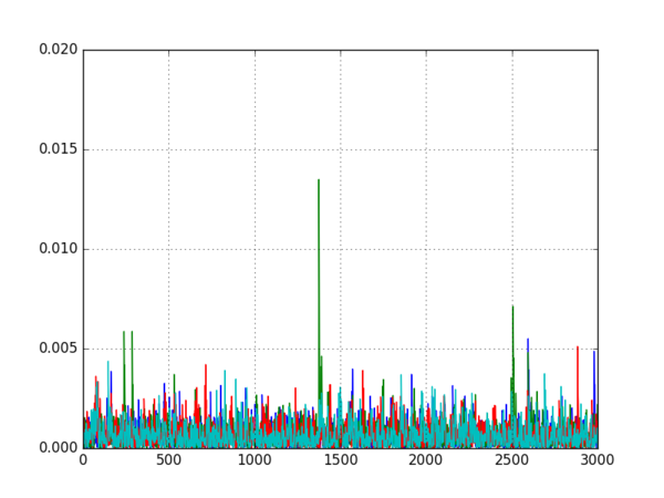
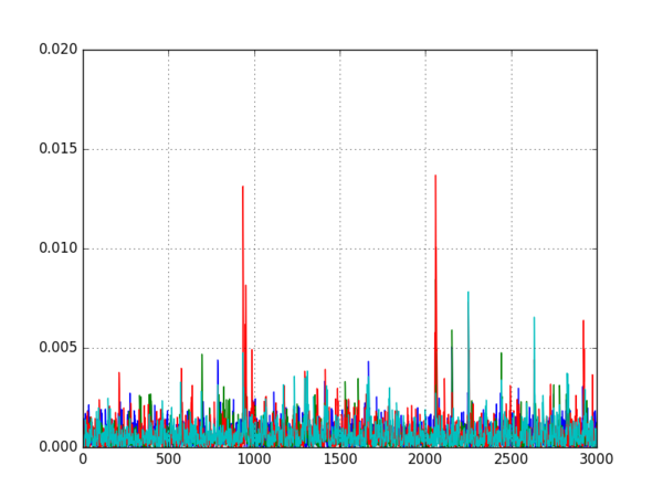
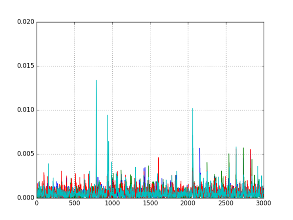
Running this script on all five datasets produced the following five graphs:
ECB:
CBC:
CFB:
OFB:
CTR:
It is quite clear from these graphs which encryption modes are being used, so the attack was successful.


