| As of August 2020 the site you are on (wiki.newae.com) is deprecated, and content is now at rtfm.newae.com. |
Difference between revisions of "Template Attacks"
(→Noise Distributions: Added plot of normal distribution) |
(→Multivariate Statistics: Added basics of multivariate stats.) |
||
| Line 44: | Line 44: | ||
== Multivariate Statistics == | == Multivariate Statistics == | ||
| − | '' | + | The 1-variable Gaussian distribution works well for one measurement. What if we're working with more than one random variable? |
| + | |||
| + | Suppose we're measuring two voltages that have some amount of noise on them. We'll call them <math>\mathbf{X}</math> and <math>\mathbf{Y}</math>. As a first attempt, we could write down a model for <math>\mathbf{X}</math> using a normal distribution and a separate model for <math>\mathbf{Y}</math> using a different distribution. However, this might not always make sense. If we write two separate distributions, what we're saying is that the two variables are independent: when <math>\mathbf{X}</math> goes up, there's no guarantee that <math>\mathbf{Y}</math> will follow it. | ||
| + | |||
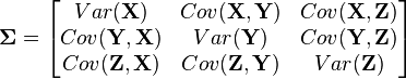
| + | Multivariate distributions let us model multiple random variables that may or may not be correlated. In a multivariate distribution, instead of writing down a single variance <math>\sigma</math>, we keep track of a whole matrix of covariances. For example, to model three random variables (<math>\mathbf{X}, \mathbf{Y}, \mathbf{Z}</math>), this matrix would be | ||
| + | |||
| + | <math> | ||
| + | \mathbf{\Sigma} = | ||
| + | \begin{bmatrix} | ||
| + | Var(\mathbf{X}) & Cov(\mathbf{X}, \mathbf{Y}) & Cov(\mathbf{X}, \mathbf{Z}) \\ | ||
| + | Cov(\mathbf{Y}, \mathbf{X}) & Var(\mathbf{Y}) & Cov(\mathbf{Y}, \mathbf{Z}) \\ | ||
| + | Cov(\mathbf{Z}, \mathbf{X}) & Cov(\mathbf{Z}, \mathbf{Y}) & Var(\mathbf{Z}) | ||
| + | \end{bmatrix} | ||
| + | </math> | ||
| + | |||
| + | Also, note that this distribution needs to have a mean for each random variable: | ||
| + | |||
| + | <math> | ||
| + | \mathbf{\mu} = | ||
| + | \begin{bmatrix} | ||
| + | \mu_X \\ | ||
| + | \mu_Y \\ | ||
| + | \mu_Z | ||
| + | \end{bmatrix} | ||
| + | </math> | ||
| + | |||
| + | The PDF of this distribution is more complicated: instead of using a single number as an argument, it uses a vector with all of the variables in it (<math>\mathbf{x} = [x, y, z, \dots]^T</math>). The equation for <math>k</math> random variables is | ||
| + | |||
| + | <math> | ||
| + | f(\mathbf{x}) | ||
| + | = \frac{1}{\sqrt{(2\pi)^k |\mathbf{\Sigma}|}} | ||
| + | e^{-(\mathbf{(x - \mu)}^T \mathbf{\Sigma}^{-1} \mathbf{(x - \mu)} / 2} | ||
| + | </math> | ||
| + | |||
| + | Don't worry if this looks crazy - the SciPy package in Python will do all the heavy lifting for us. As with the single-variable distributions, we're going to use this to find how likely a certain observation is. In other words, if we put <math>k</math> points of our power trace into <math>\mathbf{x}</math> and we find that <math>f(\mathbf{x})</math> is very high, then we've probably found a good guess. | ||
= Profiling a Device = | = Profiling a Device = | ||
Revision as of 05:13, 25 May 2016
Template attacks are a powerful type of side-channel attack. These attacks are a subset of profiling attacks, where an attacker creates a "profile" of a sensitive device and applies this profile to quickly find a victim's secret key.
Template attacks require more setup than CPA attacks. To perform a template attack, the attacker must have access to another copy of the protected device that they can fully control. Then, they must perform a great deal of pre-processing to create the template - in practice, this may take dozens of thousands of power traces. However, the advantages are that template attacks require a very small number of traces from the victim to complete the attack. With enough pre-processing, the key may be able to be recovered from just a single trace.
There are four steps to a template attack:
- Using a copy of the protected device, record a large number of power traces using many different inputs (plaintexts and keys). Ensure that enough traces are recorded to give us information about each subkey value.
- Create a template of the device's operation. This template notes a few "points of interest" in the power traces and a multivariate distribution of the power traces at each point.
- On the victim device, record a small number of power traces. Use multiple plaintexts. (We have no control over the secret key, which is fixed.)
- Apply the template to the attack traces. For each subkey, track which value is most likely to be the correct subkey. Continue until the key has been recovered.
Contents
Signals, Noise, and Statistics
Before looking at the details of the template attack, it is important to understand the statistics concepts that are involved. A template is effectively a multivariate distribution that describes several key samples in the power traces. This section will describe what a multivariate distribution is and how it can be used in this context.
Noise Distributions
Electrical signals are inherently noisy. Any time we take a voltage measurement, we don't expect to see a perfect, constant level. For example, if we attached a multimeter to a 5 V source and took 4 measurements, we might expect to see a data set like (4.95, 5.01, 5.06, 4.98). One way of modelling this voltage source is
where  is the noise-free level and
  is the additional noise. In our example, would be exactly 5 V. Then,
  is a random variable: every time we take a measurement, we can expect to see a different value. Note that
  and are bolded to show that they are random variables.
A simple model for these random variables uses a Gaussian distribution (read: a bell curve). The probability density function (PDF) of a Gaussian distribution is
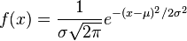
where  is the mean and
  is the standard deviation. For instance, our voltage source might have a mean of 5 and a standard deviation of 0.5, making the PDF look like:

We can use the PDF to calculate how likely a certain measurement is. Using this distribution,
so we're very unlikely to see a reading of 7 V. We'll use this to our advantage in this attack: if  is very small for one of our subkey guesses, it's probably a wrong guess.
Multivariate Statistics
The 1-variable Gaussian distribution works well for one measurement. What if we're working with more than one random variable?
Suppose we're measuring two voltages that have some amount of noise on them. We'll call them and  . As a first attempt, we could write down a model for using a normal distribution and a separate model for using a different distribution. However, this might not always make sense. If we write two separate distributions, what we're saying is that the two variables are independent: when goes up, there's no guarantee that will follow it.
Multivariate distributions let us model multiple random variables that may or may not be correlated. In a multivariate distribution, instead of writing down a single variance , we keep track of a whole matrix of covariances. For example, to model three random variables ( ), this matrix would be
Also, note that this distribution needs to have a mean for each random variable:

The PDF of this distribution is more complicated: instead of using a single number as an argument, it uses a vector with all of the variables in it (![\mathbf{x} = [x, y, z, \dots]^T](/images/math/9/2/c/92c0cda2bde551dd57b06ef9cf59e38c.png) ). The equation for
). The equation for  random variables is
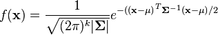
Don't worry if this looks crazy - the SciPy package in Python will do all the heavy lifting for us. As with the single-variable distributions, we're going to use this to find how likely a certain observation is. In other words, if we put points of our power trace into  and we find that
  is very high, then we've probably found a good guess.